Calibration

Note

Currently only tag model W190PD3GT is covered, but other tags will be added as opportunity permits.

Accelerometer

Note

The calibration procedure described below needs review (particularly the orientation of the sensor for the associated gravitational forces). This will be updated to be a thorough explanation in subsequent releases of the documentation.

The data provided by the Little Leonardo dataloggers are presented in a raw format which need to be adjusted to units of gravity (g). Within a period of approximately one month adjacent to collection of data, a calibration file should be created using the process described below.

Collecting calibration data

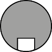
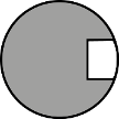
First configure and activate the datalogger for recording. For a period of approximately 10 seconds orient the tag in each of the following orientations, one axis at a time. Longer durations make visually identifying these periods in the data easier.

	+g orientation	-g orientation
X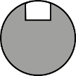
Y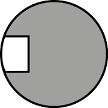
Z

Running the calibration software

Calibration is performed on accelerometer sensor data that does not have accompanying magnetometer or gyroscope data by performing by making a linear fit between a collection of points occurring at -g and +g orientations of an axis. This fit can then be applied to the original accelerometer count data to transform the data into units of g.

Launching the application

An application for simplifying the calibration process (made with the bokeh visualization library) has been included with pylleo as an executable script, which launches a bokeh application in your web-browser.

The script is automatically installed with pylleo, just run it from the command-line with an option for specifying how it opens in your browser:

Usage: pylleo-cal [OPTIONS]

  Calibrate accelerometer data

Options:
  --new TEXT  Method to open application in browser. "tab" opens the
              application in a new browser, and "window" opens it in a new
              browser window.
  --help      Show this message and exit.

The following page should appear in your browser, and the application will shut itself down when you close this page:

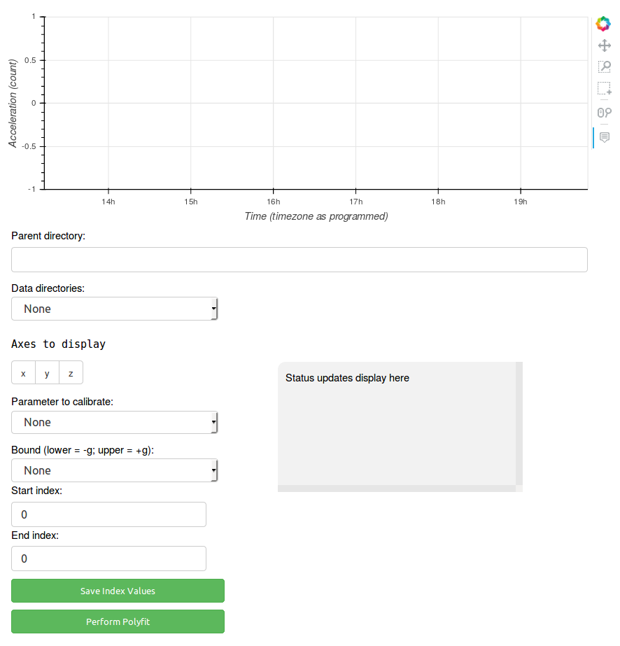
By zooming into segments of data when the datalogger was at one of the two orientations described above, a selection tool can be used to select those data points to be used for calibration. The start and stop index positions for each of these segments are saved to a file in the data directory cal.yml, and once all indices have been saved the fit coefficients can be calculated and saved to the same file. These coefficients can later be used for applying the fit to the data points using the routine lleocal.calibrate_accelerometer().

The tools for zooming and selecting the data are in the top right hand corner of the page. A summary table of the tools used in the app (shown below) have been taken from the Bokeh documentation for plot tools.

Icon	Bokeh documentation description
	The pan tool allows the user to pan the plot by left dragging the mouse or dragging a finger across the plot region.
	The box zoom tool allows the user to define a rectangular region to zoom the plot bounds too, by left-dragging a mouse, or dragging a finger across the plot area.
	The box selection tool allows the user to define a rectangular selection region by left-dragging a mouse, or dragging a finger across the plot area.
	The wheel zoom tool will zoom the plot in and out, centered on the current mouse location. It will respect any min and max value ranges preventing zooming in and out beyond these.
	The hover tool is a passive inspector tool. It is generally on at all times, but can be configured in the inspectors menu associated with the toolbar.

Loading data

All of your data should be organized in their own directories within one “parent” directory. Copy-paste the full path to this parent directory to the text input field labeled “Parent directory”.

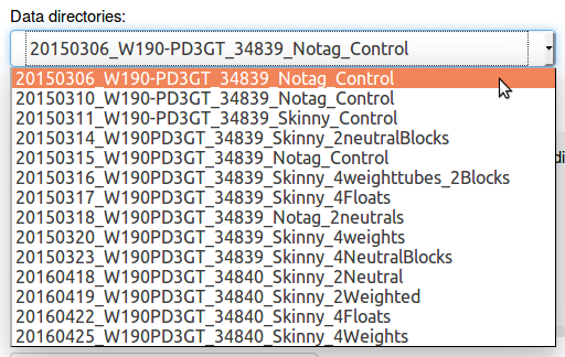
The drop-down list labeled “Data directories” will then propagate with a list of the directories in your parent directory. The data from the first directory in the list will be loaded into the plot. To select a different directory, select it from the list and its data will be loaded.

Selecting data

The app first loads all three axes of acceleration data, which from time to time may be helpful to view at the same time for comparing differences between the axes in +g/-g orientations. When selecting the index positions for the start and end of the calibration orientation regions, it is usually easiest to have only one axis displayed at a time.

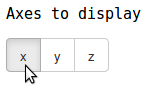
To start with the x-axis, de-select the y and z axes under the text “Axes to Display” by clicking on the buttons with their respective labels:

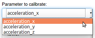
Make sure the data parameter (i.e. accelerometer axis) you wish to select calibration indices for is selected:

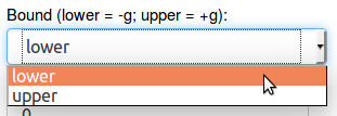
And the “bound” (i.e. the +g or -g position for that axis):

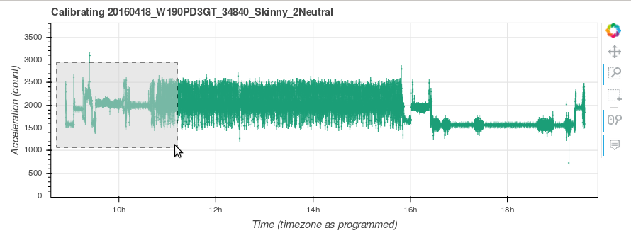
Assuming the calibration sequence was performed before the deployment of the datalogger, zoom this region of data using the tool:

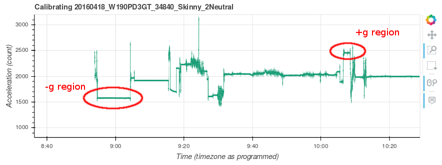
If the calibration sequence of orienting the datalogger was performed correctly, it should be obvious to see where the +g/-g positions are in the data:

Zoom in again to the region corresponding with the bound you are selecting indices for, “lower” or “upper”:

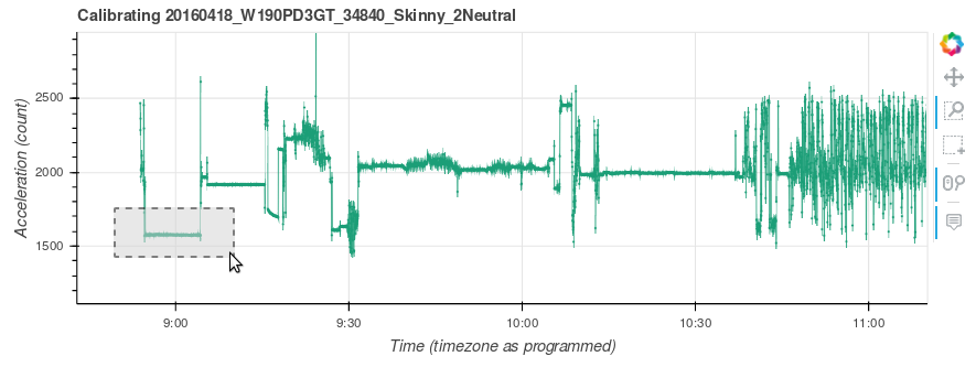
Then using the tool, click and drag across a section of data without large amounts of variation.

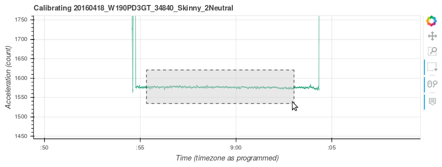
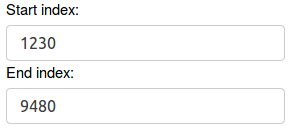
Notice that the start and end index position values have updated to the positions of the start and end of the horizontal area selected:

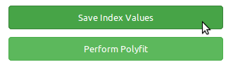
Saving the index values

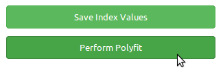
Once you have start and end index values for the region you are working with (e.g. accelerometer_x/lower), Click the button labeled “Save Index Values”:

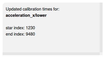
You should then see a message displayed in the gray box to the right of the selection menu letting you know that the index positions for that region saved correctly to the cal.yml. This message includes the data parameter and bound you have selected and the start and end index positions you have selected:

Once completed, you can zoom out again using the tool to perform these steps on the “upper” region. Be sure to select the correct data parameter and bound before saving the next index positions.

Then repeat these steps for the x and y axes until you have saved the index positions for all calibration orientation regions:

• acceleration_x/lower
• acceleration_x/upper
• acceleration_y/lower
• acceleration_y/upper
• acceleration_z/lower
• acceleration_z/upper

Saving the polyfit coefficients

Once you have saved all of the index positions for all calibration orientation regions, click the button labeled “Perform Polyfit”:

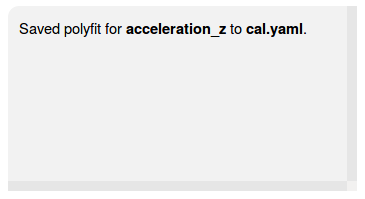
If the coefficients were able to successfully save to the cal.yml file, you should get a message in the gray box as follows:

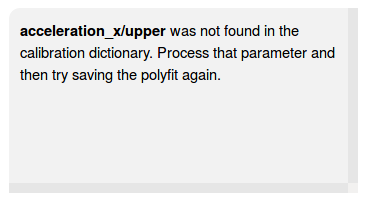
If you are missing any index positions, you will get a message indicating the first of the missing regions you must select and save before you can perform the polyfit:

Propeller

Collecting calibration data

First configure and activate the datalogger for recording. You must then move water over the datalogger’s propeller at known speeds, logging the speed of water movement, the exact start, and exact end times in spreadsheet with a preceding id column, saving it as a csv file as shown below.

As with the accelerometer file, a calibration of the propeller sensor should be performed within approximately 1 month of each deployment of the datalogger.

id,start,end,est_speed,count_average
00,start,end,speed,
...
99,start,end,speed,

Running the calibration software

With the collected data loaded using pylleo. Find the timestamp in data[‘datetimes’] closest to the logged start and end times, then calculate the average count the propeller turned between each sample.

from pylleo import lleocal

cal_fname = 'speed_calibrations.csv'

cal = lleocal.create_speed_csv(cal_fname, data)
data = lleocal.calibrate_propeller(data, cal_fname)